 RARE Technologies
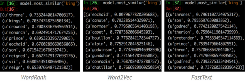 Comparisons to Word2Vec and FastText with TensorBoard visualizations.
With various embedding models coming up recently, it could be a difficult task to choose one. Should you simply go with the ones widely used in NLP community such as Word2Vec, or is it possible that some other model could be more accurate for your use case? There are some evaluation metrics which could help you to some extent in deciding a most favorable embedding model to use.
For instance, the three results above shows how differently these embeddings think for the words to be most similar to ‘king’. The WordRank results are more inclined towards the attributes for ‘king’ or we can say the words which would co-occur the most with it, whereas Word2Vec results in words(names of few kings) that could be said to share similar contexts with each other.
Here, I’ll go through some experiments for evaluating the three word embeddings, Word2Vec, FastText and WordRank and show how these different methods specialize on different downstream tasks. It primarily tells that unfortunately, there is no single global embedding model you could rely on for different types of NLP applications. You really need to choose carefully according to your final use-case.
Comparisons
The following table compares Word2Vec, FastText and WordRank embeddings in terms of their computational efficiency and accuracies on some popular NLP benchmarks. You can find the corresponding training information and hyperparameters settings used for the models, with the code to perform all the experiments below in this Jupyter notebook.
For training Word2Vec, Gensim-v0.13.3 Cython implementation was used. For training the other two, original implementations of wordrank and fasttext was used. Word2Vec and FastText was trained using the Skip-Gram with Negative Sampling(=5) algorithm. 300 dimensions with a frequency threshold of 5, and window size 15 was used.
| Algorithm | Corpus size (No. of tokens) | Train time (sec) | No. of passes for corpus | No. of cores (8GB RAM) | Semantic accuracy | Syntactic accuracy | Total accuracy | Word similarity (SimLex-999) | Word similarity (WS-353) |
| Word2Vec | 1 Million | 18 | 6 | 4 | 4.69 | 2.77 | 3.0 | Pearson: 0.17 Spearman: 0.15 |
0.37
0.37 |
| FastText | 1 Million | 50 | 6 | 4 | 6.57 | 36.95 | 32.9 | Pearson: 0.13 Spearman: 0.11 |
0.36
0.36 |
| WordRank | 1 Million | ~4 hours | 91 | 4 | 15.26 | 4.23 | 5.7 | Pearson: 0.09 Spearman: 0.10 |
0.39
0.38 |
| Word2Vec | 17 Million | 402 | 6 | 4 | 40.34 | 41.48 | 41.1 | Pearson: 0.31 Spearman: 0.29 |
0.69
0.71 |
| FastText | 17 Million | 942 | 6 | 4 | 25.75 | 57.33 | 45.2 | Pearson: 0.29 Spearman: 0.27 |
0.67
0.66 |
| WordRank | 17 Million | ~42 hours | 91 | 4 | 54.52 | 39.83 | 44.7 | Pearson: 0.29 Spearman: 0.28 |
0.71
0.72 |
You can also now use the python wrapper around WordRank which I’ve have added to gensim as part of my Incubator Project. It has functions for training, sorting and ensemble the WordRank embeddings. Here’s an introductory notebook on using the wrapper.
The two evaluations performed here used the following benchmarks:
- Google analogy dataset for Word analogies, is used that contains around 19k word analogy questions, partitioned into semantic and syntactic questions. The semantic questions contain five types of semantic analogies, such as capital cities(Paris:France;Tokyo:?) or family (brother:sister;dad:?). The syntactic questions contain nine types of analogies, such as plural nouns (dog:dogs;cat:?) or comparatives (bad:worse;good:?).
- And for Word similarity, two datasets SimLex-999 and WS-353 containing word pairs together with the human-assigned similarity judgments are used. These two datasets differ in their sense of similarities as SimLex-999 provides a measure of how well the two words are interchangeable in similar contexts, and WS-353 tries to estimate the relatedness or co-occurrence of two words. For example these two word pairs illustrate the difference[1]:
| Pair | Simlex-999 rating | WordSim-353 rating |
| coast – shore | 9.00 | 9.10 |
| clothes – closet | 1.96 | 8.00 |
Here clothes are not similar to closets (different materials, function etc.) in SimLex-999, even though they are very much related.
Now coming to the table, the main observation that can be drawn is the specializing nature of embeddings towards particular tasks, as you can see the significant difference FastText makes on Syntactic Analogies, and WordRank on Semantic ones. This is due to the different underlying approaches they use. FastText incorporates the morphological information about words. On the other hand, WordRank formulates it as a ranking problem. That is, given a word w, it aims to output an ordered list (c1, c2, · · ·) of context words such that the words that co-occur most with w appear at the top of the list. It does so by applying the ranking loss to be most sensitive at the top of context words list (where the rank is small) and less sensitive at the lower end of the list (where the rank is high).[2]
And for the Word Similarity, Word2Vec seems to perform better on SimLex-999 test data, whereas, WordRank performs better on WS-353. This is probably due to the different types of similarities these datasets address. The list outputs above of most similar words to ‘king’ also showed a notable difference of the way these embeddings think of similarity.
Visualizing the Embeddings
Now we’ll try to visualize the three embeddings using TensorBoard. But as we go through the visualizations of different embeddings below, you would observe that they mostly try to replicate the list outputs of most_similar for ‘king’ which we saw in the beginning. We don’t really get any new insights into the differences between these embeddings from visualization, that we couldn’t get from the most_similar lists above.
The multi-dimensional embeddings are downsized to 2 or 3 dimensions for effective visualization. We basically end up with a new 2d or 3d embedding which tries to preserve information from the original multi-dimensional one. As the word vectors are reduced to a much smaller dimension, the exact cosine/euclidean distances between them are not preserved, but rather relative, and hence as you’ll see below the nearest similarity results may change.
TensorBoard provides two popular dimensionality reduction methods for visualizing the dataset.
- Principal Component Analysis (PCA) which tries to preserve the global structure in the data, and due to this local similarities of data points may suffer in few cases. You can see an intuition behind it in this nicely explained answer on stackexchange.
- The next one, t-SNE, which tries to reduce the pairwise similarity error of data points in the new space. That is, instead of focusing only on the global error as in PCA, t-SNE try to minimize the similarity error for every single pair of data points. You can refer to this blog, which explain about its error minimization and how similarities are constructed.
See this doc for instructions on how to use TensorBoard. You can also use this already-running TensorBoard, and upload the TSV files containing word embeddings. I’ve provided the link to my uploaded model’s projector config and also the TSV files used for it.
 2D PCA results for Word2Vec 2D t-SNE results for Word2Vec
Word2Vec model link: w2v_projector_config
TSV files: https://github.com/parulsethi/EmbeddingVisData/tree/master/Word2Vec
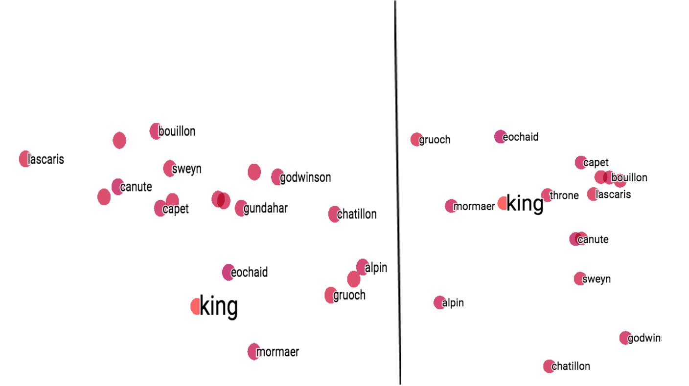
The figures above show the results for both PCA and t-SNE. In Word2Vec case, both methods perform fine in placing results relative to ‘king’ and PCA ends up covering 84% variance in data. Now if you go to the model link and try using t-SNE, you may get some different results as t-SNE is a stochastic method, and might have multiple minima that lead to different solutions. So the results may differ even if you use the same parameter settings as mine (mentioned below). You can see this thread for some differences between both methods.
 2D PCA results for FastText 2D t-SNE results for FastText
Fasttext model link: ft_projector_config
TSV files: https://github.com/parulsethi/EmbeddingVisData/tree/master/FastText
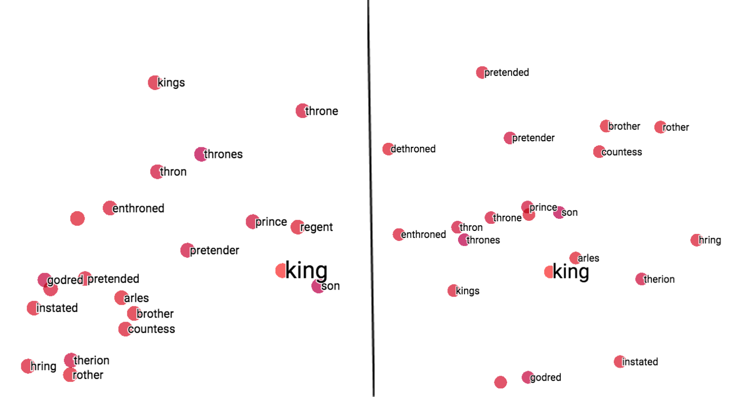
For FastText, both the methods performed similar, but the results were little inferior than that of Word2Vec in placing the words according to their similarity order.
 2D PCA results for WordRank 2D t-SNE results for WordRank
WordRank model link: wr_projector_config
TSV files: https://github.com/parulsethi/EmbeddingVisData/tree/master/WordRank
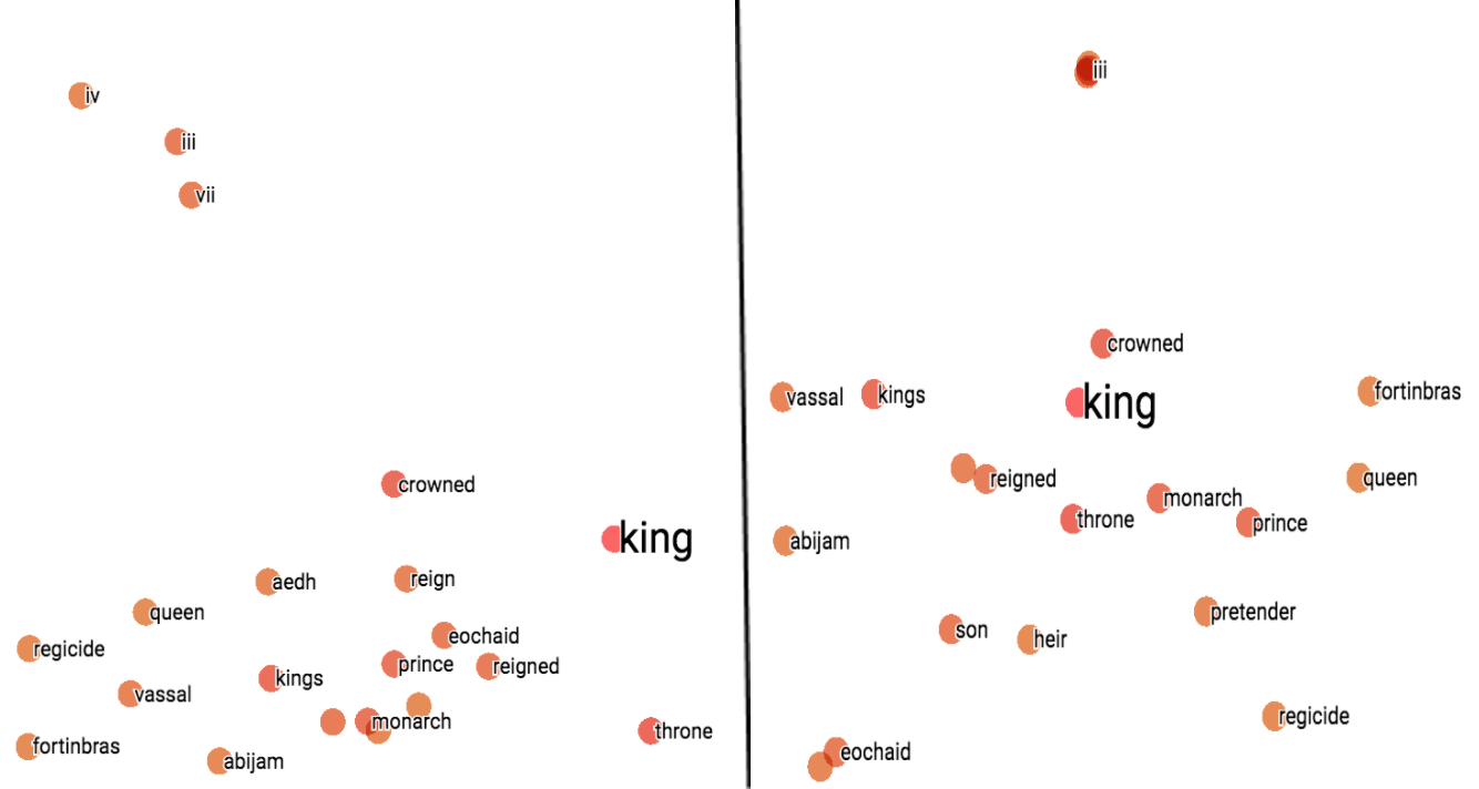
For WordRank, t-SNE results seems to be slightly better than PCA’s, as in PCA, some top similar results got placed comparatively far. Probably, because PCA covers 58% variance in this case which is also the lowest amongst all models.
Now t-SNE can be a bit tricky to use, and you should really read this article before using it for any interpretation of your data. As for generating the above visualizations from t-SNE, I used the perplexity value of 10, learning rate 10, iteration count of 500 till which all three models stabilized to a particular configuration, and isolated my data to 20 most similar points around the word ‘king’. Also, there’s an option to normalize the data by using ‘Sphereize data’ but that could change few results in the original space, so it wasn’t used for the above visualizations.
Note: You can also use gensim to convert your word vector files to TSV format and then simply upload them to http://projector.tensorflow.org/ to generate this visualization.
WordRank Hyperparameter tuning
Now, before going to the next part of evaluation, I’d like to put some light on an important aspect of WordRank that when it comes to tuning the hyperparameters, WordRank generally performs better with its default values only that are provided in its demo and is not extremely sensitive to that as compared to the other embedding models. These are some of the explored values for WordRank and their optimal cases.
| Hyperparameter | Explored Values | Optimal performing cases |
| Window size | 5, 10, 15 | small window sizes decrease the accuracy for both word similarity and analogy tasks, and word rank performed optimum with a value of 15 |
| w+c ensemble | -w, -w+c | while ensemble of word and context embeddings improve accuracy in small corpus, it doesn’t help in large corpus and effects accuracy negatively. (This is a Post-training hyperparameter explained below in detailed word analogy experiment) |
| Epochs | 50, 100, 500 | As word rank is very time consuming, it may not be feasible to do 500 epochs which is default, so you can also go with 100 epochs which give somewhat comparable results. |
| Learning Rate | 0.001, 0.025 | large learning rate results in diverged embeddings and too small value could take very long for convergence given wordrank is already very time consuming |
Word Frequency and Model Performance
In this section, we’ll see how Embedding model’s performance in Analogy task varies across the range of word frequency. Accuracy vs. Frequency graph is used to analyze this effect.
The mean frequency of four words involved in each analogy is computed, and then bucketed with other analogies having similar mean frequencies. Each bucket has six percent of the total analogies involved in the particular task. You can go to this repo if you want to inspect about what analogies(with their sorted frequencies) were used for each of the plot.
For 1 million tokens (Brown corpus):
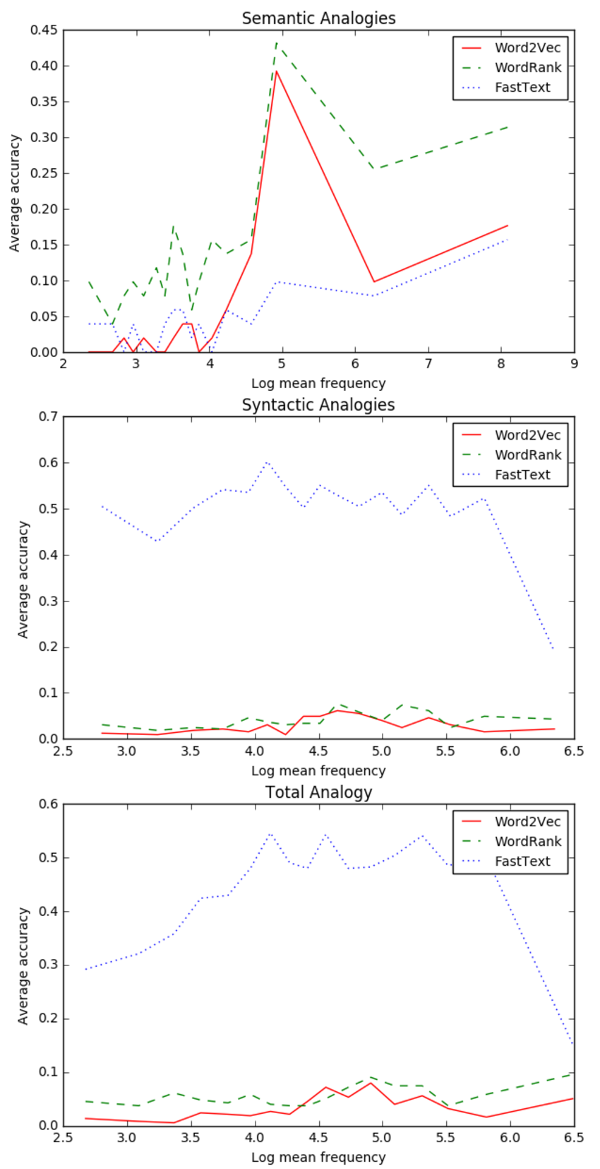
The main observations that can be drawn here are-
- In Semantic Analogies, all the models perform poorly for rare words as compared to their performance at more frequent words.
- In Syntactic Analogies, FastText performance is way better than Word2Vec and WordRank.
- If we go through the frequency range in Syntactic Analogies plot, FastText performance drops significantly at highly frequent words, whereas, for Word2Vec and WordRank there is no significant difference over the whole frequency range.
- End plot shows the results of combined Semantic and Syntactic Analogies. It has more resemblance to the Syntactic Analogy’s plot because the total no. of Syntactic Analogies(=5461) is much greater than the total no. of Semantic ones(=852). So it’s bound to trace the Syntactic’s results as they have more weightage in the total analogies considered.
Now, let’s see if a larger corpus creates any difference in this pattern of model’s performance over different frequencies.
For 17 million tokens (text8):
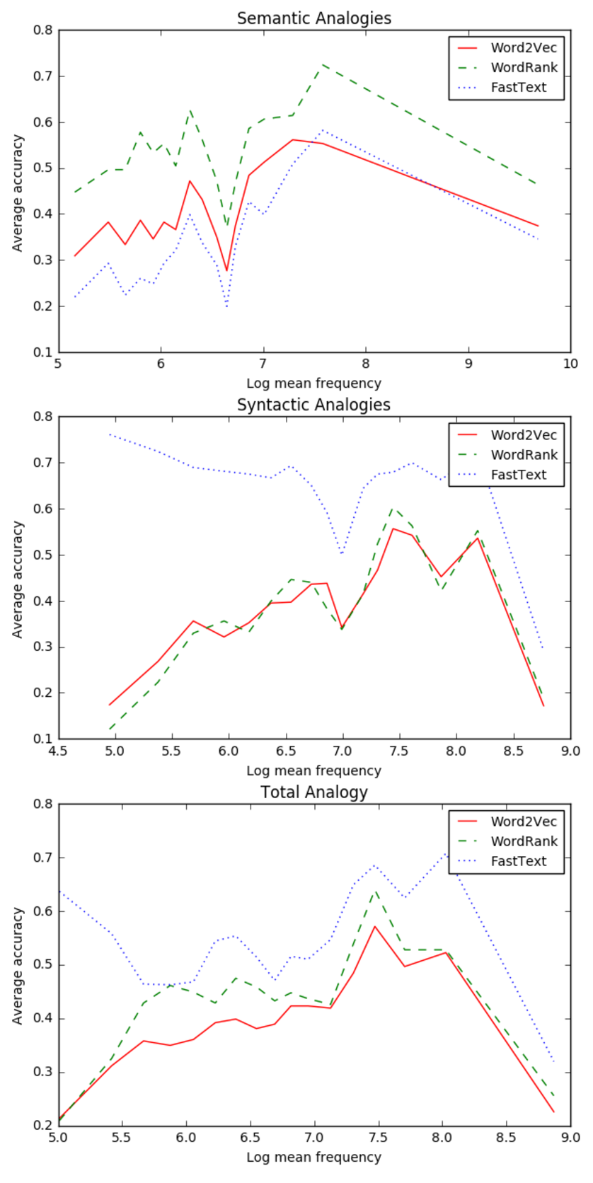
Following points can be observed in this case-
- For Semantic analogies, all the models perform comparitively poor on rare words and also when the word frequency is high towards the end.
- For Syntactic Analogies, FastText performance is fairly well on rare words but then falls steeply at highly frequent words.
- WordRank and Word2Vec perform very similar with low accuracy for rare and highly frequent words in Syntactic Analogies.
- FastText is again better in total analogies case due to the same reason described previously. Here the total no. of Semantic analogies are 7416 and Syntactic Analogies are 10411.
These graphs also conclude that WordRank is the best suited method for Semantic Analogies, and FastText for Syntactic Analogies for all the frequency ranges and over different corpus sizes, though all the embedding methods could become very competitive as the corpus size largerly increases[3].
Word Analogies
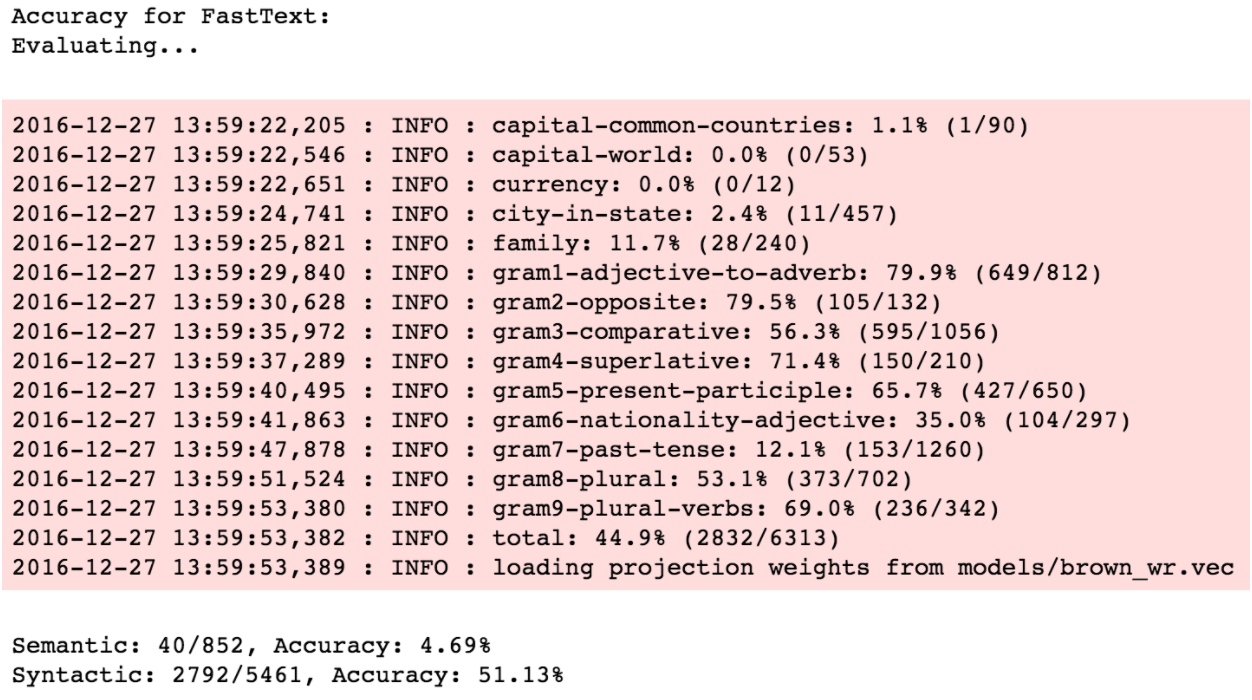
This section provides the detailed logs of embedding models on Analogy task that shows the accuracies for different analogy categories. This will also show how these embeddings perform differently on Semantic and Syntactic Analogies.
The first comparison is on 1 million tokens (brown corpus).
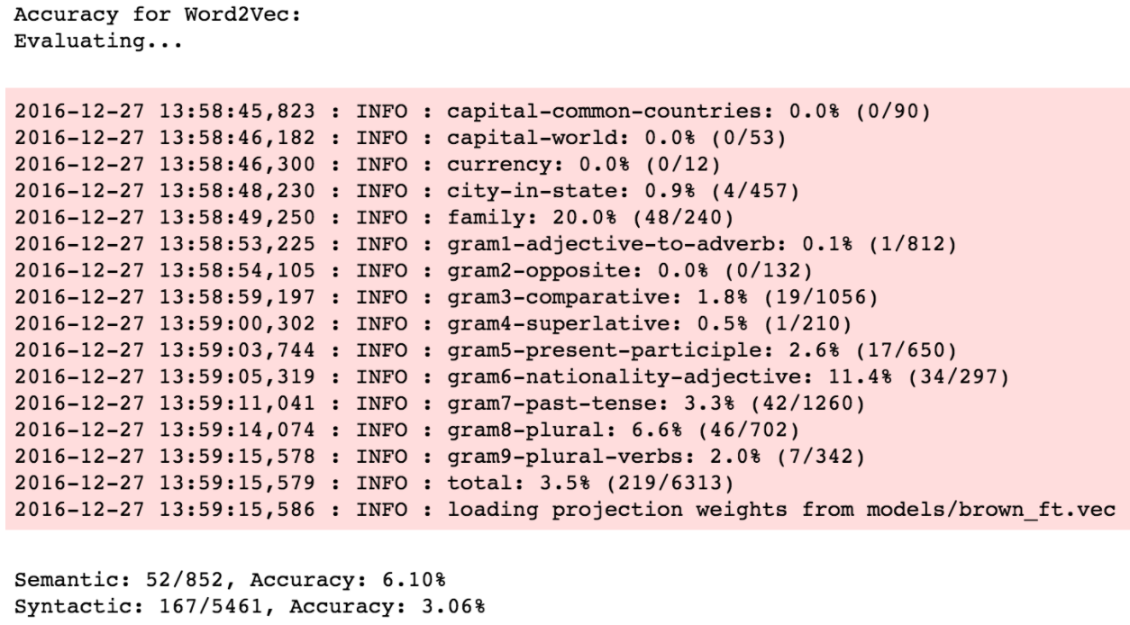
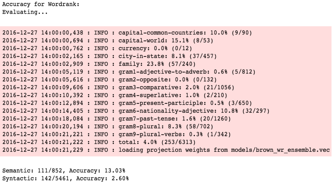
Now, WordRank generates two sets of embeddings, word and context embeddings. Former one is for vocabulary words and latter for the context words. WordRank models the relation between them using their vector’s inner product which should be directly proportional to their mutual relevance i.e. the more relevant the context is, the larger should be its inner product with the vocab word. This formulation helps in the case where you need to model the semantic relatedness in your data, i.e., how often the two words co-occur.
So, let’s try the ensemble, which is basically a post-training hyperparameter and adds the two sets of vectors generated. For example, word “cat” can be represented as:
![]() where ~w and ~c are the word and context embeddings, respectively.
where ~w and ~c are the word and context embeddings, respectively.
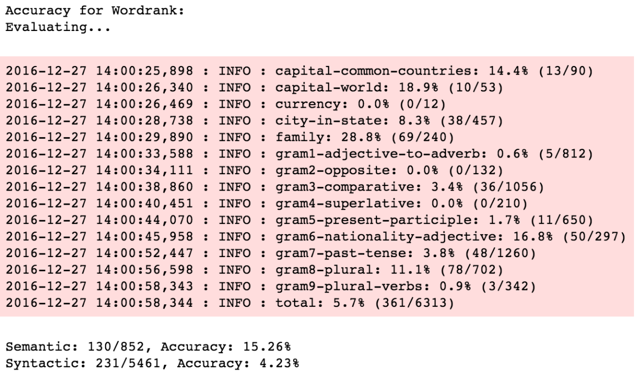
This vector combination, called ensemble method, generally helps reduce overfitting and noise and gives a small performance boost (Ciresan et al., 2012) and the same is apparent from the results of ensemble embedding here.
Now, let’s evaluate these algorithms on a large corpus, text8, which is a preprocessed sample of wikipedia data.
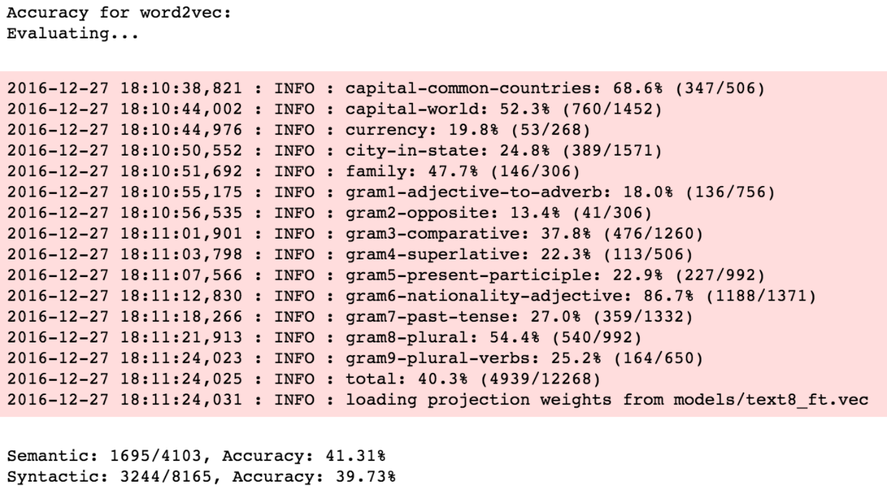
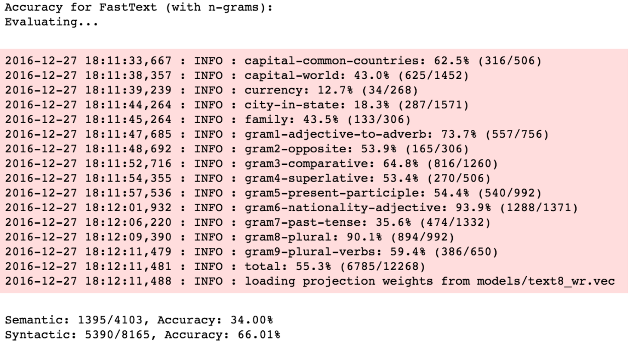
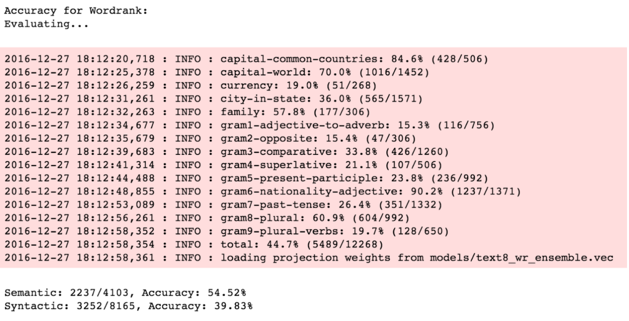
With the text8 corpus, we observe a similar pattern. WordRank again performs better than both the other embeddings on semantic analogies, whereas, FastText performs significantly better on syntactic analogies.
Note: WordRank can sometimes produce NaN values during model evaluation, when the embedding vector values get too diverged at some iterations, but it dumps embedding vectors after every few iterations, so we can just load embeddings from a different iteration’s text file.
Conclusion
The experiments here conclude two main points about comparing Word embeddings. Firstly, there is no single global embedding model we could rely on for different types of NLP applications. For example, in Word Similarity, WordRank performed better than the other two algorithms for WS-353 test data whereas, Word2Vec performed better on SimLex-999. This is probably due to the different type of similarities these datasets address as explained in task intro above. And in Word Analogy task, WordRank performed better for Semantic Analogies and FastText for Syntactic Analogies. This basically tells that we need to choose the embedding method carefully according to our final use-case.
Secondly, frequency of our query words do matter apart from the generalized model performance. As we observed in Accuracy vs. Frequency graphs that models perform differently depending on the frequency of question analogy words in training corpus. For example, we are likely to get poor results if our query words are all highly frequent.
Thanks
I am thankful to Lev for guiding me throughout this project and teaching me the know-hows of Word Embeddings. I also appreciate the valuable feedbacks from Jayant and Radim for this blog.
