 RARE Technologies
As a part of the RARE incubator program my goal was to add two new features on the existing TF-IDF model of Gensim. One was implementing a SMART information retrieval system (smartirs) scheme [1] and the other was implementing pivoted document length normalization [2].
In this blog I'll discuss the whys and whats of the implementation. I'll also inspect the original paper by Singhal, et al [2] on pivoted document length normalization.
Why pivoted document length normalization?
When classifying documents into various categories it was noticed in the same paper Singhal, et al [2] that cosine normalization tends to favor retrieval of short documents but suppresses the retrieval of long documents:
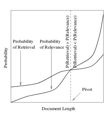
Figure 1. - The variation of probability of retrieval and relevance with respect to document length.
Our goal is to boost the probability of retrieving long documents and suppress the probability of retrieval of short documents so that the probability of retrieval and relevance for a given document align.
101 on TF-IDF
Before we get to pivoted normalization itself, a few words on the bag-of-words model, term-frequency-inverse-document-frequency (TF-IDF) and the SMART weighting schemes. If you’re familiar with TF-IDF and its variants, you can skip straight to the sections below.
Term glossary
Term Frequency is the number of times a word has occurred in the document or a words frequency in a document. Its domain remains local to the document. Document frequency is the fraction of documents in which the word has occurred. It’s calculated based on statistics collected from the entire corpus.
In very simple terms TF-IDF scheme is used for extracting features or important words which can be the best representative of your document. To get the intuitive feel of TF-IDF, consider a recipe book which has recipe of various fast foods.
Here the recipe book is our corpus and each recipe is our document. Now consider various recipes such as:
- Burger which will consist of words like "bun", "meat", "lettuce", "ketchup", "heat", "onion", "food", "preparation", "delicious", "fast"
- French fries which will consist of words like "potato", "fry", "heat", "oil", "ketchup", "food", "preparation", "fast"
- Pizza which will consist of words like "ketchup", "capsicum", "heat", "food", "delicious", "oregano", "dough", "fast"
Here words like "fast", "food", "preparation", "heat" occur in almost all the recipes. Such words will have a very high document frequency. Now consider words like "bun", "lettuce" for the recipe burger, "potato" and "fry" for the recipe french fries and "dough" and "oregano" for the recipe pizza. These have a high term frequency for the particular recipe they are related to, but will have a comparatively low document frequency.
Now we propose the scheme of TF-IDF which simply put is a mathematical product of term-frequency and inverse of the document frequency of each term. One can clearly visualize how the words like "potato" in French fries will have a high TF-IDF value and at the same time are the best representative of the document which in this case is "French Fries".
Now mathematically speaking:
-
Term frequency: For a word (or term)
t, the term frequency is denoted bytft,dand the frequency of each term in a documentdis denoted byft,dthentft,d = ft,d -
Inverse document frequency: Taking the log smartirs scheme for inverse document frequency
idfis calculated asor the log of inverse fraction of document that contain the term
t, whereNis the total number of documents in the corpus. To avoid division by zero error generally 1 is added to the denominator. TF-IDF: Finally, TF-IDF is calculated as the product of term frequency
tft,dand inverse document frequencyidf(t,D),TF-IDF(t,d,D) = tft,d * idft,DRetrieval curve: It is the probability distribution of a document that is returned by the model against the document length of the documents. Refer to Figure 1.
Relevance curve It is the probability distribution of a document that is expected from the model against the document length of the documents. Refer figure 1.
Pivot: In figure 1 pivot is the document length below which the probability of retrieval is higher than the probability of relevance of a document and above which the probability of relevance is higher than the probability of retrieval of a document.
Slope: The slope decides the amount of "tilting" at the pivot point which is required to bring the relevance and retrieval curves as close as possible. Mathematically, slope is the tangent of the angle made by old normalization with the new normalisation.
SMART Information Retrieval System
There exist multiple variants of how to weight the terms and document frequencies, using subtly different formulas. To make the notation scheme clearer, describes SMART (System for the Mechanical Analysis and Retrieval of Text, see Wikipedia [1] information retrieval system, or SMARTIRS in short, defines a mnemonic scheme for denoting TF-IDF weighting variants in the vector space model. This notation is a 3-letter string of form TDN where T represents the term weighting for term frequency, D represents the term weighting for document frequency, and N represents the normalization scheme employed after the calculation of TF-IDF:
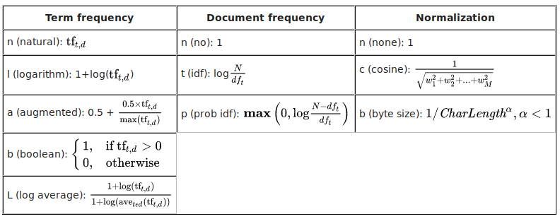
The standard SMARTIRS notation.
For example, the most basic TF-IDF variant is described as “ntc” under this scheme.
Pivoted document length normalization
With the basics out of the way, what is pivoted normalization exactly and how does it work?
We can solve the problem described in section 2 by introducing a new bias in favor of long documents to counter the unwanted bias introduced by cosine normalization for short documents. So our pivoted normalization scheme should be something like:
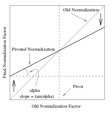
Figure 2. - Using pivot and alpha to "tilt" the old normalisation.
The normalization factor should be high for short documents and low for long documents. (Remember that the graph is plotted for calculating the normalization factor. The higher the normalization factor, the lower is the TF-IDF value. More discussion on this in the later part.)
This approach requires two parameters for the normalization to work:
We expect the user to supply both of these values. Generally, we can use the average number of unique terms in a document (computed across the entire collection) as the pivot and use grid search to get the optimum value of slope which ranges from 0 to 1. For a more detailed example the user can check this notebook out.
Using basic coordinate geometry (which we are not going to discuss here) we can propose the new normalization scheme as pivoted normalization = (1.0 - slope) x pivot + slope x old normalization.
Comparative study
I used the publicly available twenty-newsgroup dataset for comparing the traditional TF-IDF methods with that of pivoted normalization.
The study was conducted for binary classification of text into two categories namely 'sci.electronics' and 'sci.space'. The data consisted of 1184 training documents and 787 test documents belonging to the two categories.
I used TF-IDF to generate features from documents which were later fed to a logistic regression classifier. The logistic regression classifier implementation of sklearn assigns scores to each document, which for my particular case had a varying score from approximately -2 to 2. The magnitude suggests the confidence level of the model that a particular document belongs to a particular class and the sign of these scores suggested the category to which the documents should belong.
The idea was to plot a histogram for the top K scoring documents and visualize their scores.
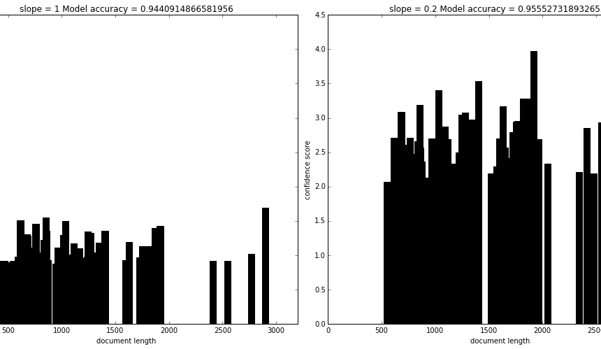
Figure 3. - The confidence scores of documents plotted against the corresponding document length. The first plot is using the traditional TFIDF and the second is using pivoted document length normalisation.
We observe an overall increase in the confidence score since we are introducing an additional bias for long documents along with the already present intrinsic bias for short document.
Also please do not confuse that the score of the same document is increased. The plot is plotted against the score of top-k documents which are different in both the plots.
In the first histogram we can see that using regular TF-IDF implementation (or when slope was 1), there was a certain bias for short documents as one can see sparsity in bins around the length of 2500 and high density of bins around the length less than and around 500. Suggesting that shorter documents had a higher probability of appearing in the top K documents.
As we decreased the slope to 0.2, we notice that the histogram plot is now equalized and shows little sign of bias with respect to document length. We also notice an increase in accuracy of 1.1%.
Also by using pivoted document normalization we notice an increase in scores of nearly all the top K documents fetched. This mostly doesn't affect our results because the scores are almost evenly scaled up. Though this suggests that our model is now more confident in classifying the documents into a particular class.

Figure 4
Figure 4 is a plot between slope and achieved accuracy of the model, it suggests that a decrease in slope doesn't always necessarily increase the accuracy. The reason for this behaviour can be attributed to the fact that by introducing too much bias for long documents to counter the bias for short documents, after a certain extent we are introducing another overall bias in the TF-IDF model which is redundant and unwanted.
