 RARE Technologies
Have you heard about the new open source Bounter Python library in town? In case you can’t wait to use it in practice but are wary of its “frequency estimation”, and what kind of results you can expect, this series of blog posts will help you develop the right intuition. It is split into two parts, one for each of the two very different algorithms we implemented in Bounter: the Count-Min Sketch (CMS) and the HashTable.
Our tale begins with a straightforward problem. We needed to count frequencies of words in a large corpus, such as the Wikipedia. We started with Python code that looked a lot like this:
from collections import Counter
from smart_open import smart_open

wc = Counter()
# preprocessed words, one Wikipedia article per line
with smart_open('wiki_tokens.txt.gz') as wiki:
    for line in wiki:
        words = line.decode().split()
        wc.update(words)
All developers rely heavily on abstract data structures. We need them to do their job effectively for simple operations, so we can focus on the complexity of our own tasks. When used like this, Python’s built-in Counter is actually pretty effective. It uses an optimized hashtable under the hood to store the key-value pairs.
However, when working with very large data sets, even this implementation has its limits. We are storing Python objects, and Python strings and integers come with a hefty memory overhead. On average, a Counter entry uses around 100 bytes.
Thus, for our Wikipedia data set with 7,661,318 distinct words, we need 800 MB just to count their frequencies. We could still work with that, but we quickly run out of excuses for bigrams: it takes 17.2 GB to count all 179,413,989 distinct word pairs. And we need those frequencies to trim model dictionaries in word2vec, LSI, LDA (and pretty much any other machine learning algorithm that works with text), to identify common phrases for collocations and so on. And Wikipedia isn’t even a particularly big dataset. We can do better!
Our team looked for ways to optimize this part of the algorithm. The original solution in Gensim was to delete the lowest-frequency entries whenever the dictionary grew too large, increasing the threshold for deletion on each prune (a technique inspired by Mikolov’s word2vec implementation). This was possible as we didn’t need the exact counts. The quality of the output was satisfactory: the long vocabulary tail is not relevant for determining good quality words or phrases. Sadly, the solution wasn’t perfect. A pruning routine written on top of Counter couldn’t be very fast, and the structure still used 100B per each entry.
We decided that we could implement the same idea much more efficiently. The first Bounter implementation, HashTable, was born.
HashTable Discarding Keys with Low Frequencies
HashTable is a frequency estimator (counter) for strings implemented as a Python C-extension. It is a fixed-size hashtable which maintains its own statistics and prunes its lowest-frequency entries automatically when it becomes too full. Furthermore, it optimizes string storage (as C strings) to use memory much more efficiently than Counter (32B per entry rather than 100B).
Initialization and size
To init this fixed-size structure, we need to set the number of buckets:
from bounter import HashTable
counts = HashTable(buckets=4194304)
One bucket takes 16B, plus we need additional memory to store the strings. In practice, this totals to around 32B per bucket on real data. Therefore, our HashTable with 4M buckets will grow to around 128MB in production, depending on average length of the stored keys. For humans, we added a more convenient API that chooses the bucket size based on this built-in knowledge:
from bounter import bounter
counts = bounter(size_mb=128)
You can always verify the number of buckets as well as the currently allocated memory:
print(counts.buckets())
4194304
print(counts._mem())  # includes string heap size (currently empty)
67109888  # 64MB
Operations
From the start, we wanted the HashTable to work as a Counter replacement, to make switching between the two easier, so we made it support most of the standard dictionary methods. For efficiency, we also added some new ones:
# Python 2
counts.update(['a', 'b', 'c', 'a'])
counts.increment('b')
# increment('b', 2) would work too!
print(counts['a'])
2
# maintains an exact tally of all increments
print(counts.total())
5
# estimate for the number of distinct keys (uses HyperLogLog)
print(counts.cardinality())
3
# currently stored elements
print(len(counts))
3
# iterator returns keys, just like Counter
print(list(counts))
[u'b', u'a', u'c']
# supports iterating over key-count pairs, etc.
print(list(counts.iteritems()))
[(u'b', 2L), (u'a', 2L), (u'c', 1L)]
You might notice something funny about the output. We updated the counter with strings (bytes objects) and we could query their count just right, but iteration gives us back unicode objects. Bounter does not care about the input string format and it stores the strings as UTF-8 bytes internally. We had to make a choice about the output (iteration) format and we decided that unicode would be a better default choice for both Python2 and Python3. If you would rather work with bytes, you can initialize the HashTable with a special parameter use_unicode=False:
counts = HashTable(buckets=64, use_unicode=False)
counts.update(['a', 'b', 'c'])
print(list(counts))
['b', 'a', 'c']  # bytes objects
HashTable is very fast (slightly faster than Python’s built-in Counter) but you should still be smart about the usage:
counts['SLOW'] += 2  # DON'T USE THIS! Counts correctly, but is much slower
counts.increment('fast', 2)  # preferable
This is because Python translates += into successive get and set operations, which are literally double the work of a hashtable lookup. Use the increment() or update() methods instead.
You may be wondering about the difference between using len() and cardinality(). len(counts) returns the number of keys that are currently stored in the HashTable, those that you get when iterating over its keys. It does not include the removed elements.
On the other hand, cardinality() is an estimate for the size of the full set (including the removed elements). This is actually a really hard thing to track after the table has been pruned more than once. Fortunately, someone had already solved it for us and we have included a hyperloglog structure in Bounter. Bounter estimates the total number of distinct keys with error less than 1% now.
Likewise, the total() method returns a sum of all counts including the removed entries. This tally is precise, not an estimate, because keeping track of that is straightforward.
Hashtable pruning
With the basics out of the way, you may be anxious to know how pruning works and how it behaves in practice.
Just like an ordinary dictionary, when 3/4 of HashTable’s buckets are filled, it needs to free some space. An ordinary hashtable-based dictionary expands itself by doubling the bucket array. Instead, HashTable removes entries with low counts. Before doing so, it needs to find the best threshold value. Pruning is an operation linear in the size of the structure and we don’t want to do it too often. To this end, HashTable maintains a simple histogram of stored frequencies. It consults the histogram to find the lowest threshold so that at least ⅓ of the entries are removed, leaving the table at most 50% full. As we are always pruning a large fraction of all keys, the pruning operation is sufficiently amortized among the inserts and the structure maintains an amortized constant complexity for its operations.
Let’s look at the counting accuracy now. As long the number of distinct elements is less than 3/4 of the buckets, all counts are exact. When the cardinality goes above this number, pruning decreases some counts. This means HashTable’s frequency estimates are biased: they might underestimate, but never overestimate. Keys with high frequencies are unlikely to be affected by pruning, although it can happen, particularly for keys that are unevenly distributed in the input stream (a lot of occurrences by the end of the input but occur only sporadically near the beginning).
The following chart visualises this effect:
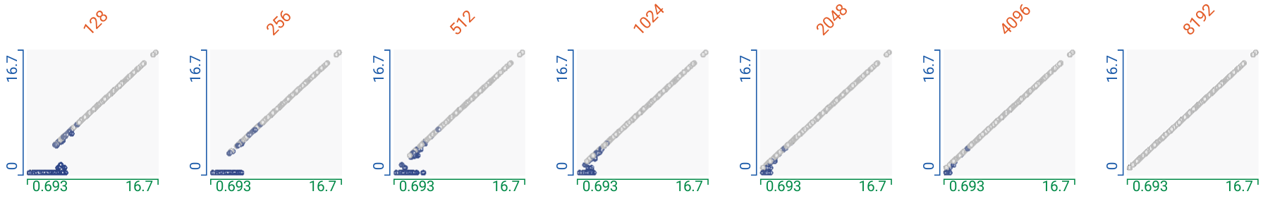
Each subchart shows one Bounter instance which was used to count frequencies of all bigrams from the English Wikipedia (179M distinct). Above the chart is the value of the size_mb parameter used to initialize the Bounter structure. We took a sample of 500 random bigrams and drew a scatterplot using their actual (log-scaled x-axis) and Bounter-estimated (log-scaled y-axis) frequencies. The color of the dot is darker when the estimate is not correct.
The chart shows the effect of pruning: most of the elements beneath a certain threshold return 0, or another low value, yet values above that threshold are mostly precise except for a few which are underestimated by a very small margin. From left to right, you can very clearly follow the improvement in result accuracy, as we allot more and more memory to Bounter.
If you want to see the charts in action and explore its individual data points, click here to open the chart in a new FacetsDive window. You can read more on interactive analytics with Google’s FacetsDive tool in our recent tutorial.
| Bounter size | buckets() | quality() | precision | recall | F1 |
|---|---|---|---|---|---|
| 128MB | 4M | 42.78 | 1.0 | 0.847 | 0.917 |
| 256MB | 8M | 21.39 | 1.0 | 0.909 | 0.952 |
| 512MB | 16M | 10.69 | 1.0 | 0.956 | 0.978 |
| 1024MB | 32M | 5.34 | 1.0 | 0.993 | 0.996 |
| 2048MB | 64M | 2.67 | 1.0 | 1.0 | 1.0 |
| 4096MB | 128M | 1.34 | 1.0 | 1.0 | 1.0 |
| 8192MB | 256M | 0.89 | 1.0 | 1.0 | 1.0 |
After counting a large data set with Bounter, you might be interested in the degree of degradation of results. The quality() method returns a ratio of the estimated cardinality and its capacity. In other words, how much more memory you would need for precise results.
counts = HashTable(buckets=8) # can store at most 6 items
counts.update(['a', 'b', 'c'])
print(counts.quality()) # 0.5, or 3/6
counts.update(['d', 'e', 'f', 'g', 'h', 'i'])
print(counts.quality()) # 1.5, or 9/6
Evaluation
Finally, we checked whether the accuracy is good enough for our original purpose, extracting collocations (common phrases) from the English Wikipedia. We took a random sample of 2000 bigrams and checked which of them evaluate as phrases using a Counter with exact values (27.5% of them did). Then we used the same algorithm to determine the phrases, but this time using the estimated counts from Bounter. We compared whether the result was the same for each bigram and calculated precision, recall, and F1 values, which you can see in the table below the chart.
Unsurprisingly, HashTable had a perfect precision score in all cases. This is because the results are never overestimated, so all reported phrases were true positives. The number of false negatives increased as we decreased the memory, with more and more small values being underestimated as 0 (or a very low number).
As you can see, even with a significantly reduced memory, HashTable gives us great performance for phrases generation. With just 128MB, 137x less memory than that is required by Python’s Counter, we managed a very respectable recall of 84.7%.
Of course, these results could only be achieved because of the “long tail” property of our data: most elements had a really small frequency whereas there were considerably less elements with higher frequency. In our NLP domain, this data property holds (Zipf’s law) but you have to be mindful if applying Hashtable elsewhere.
Stay tuned for the next post, where we take a similar look at CountMinSketch, the second algorithm in Bounter, which takes this result even further, using a completely different data structure and trade-offs.
