 RARE Technologies
I have been working on implementing a model called Poincaré embeddings over the last month or so. The model is from an interesting paper by Facebook AI Research – Poincaré Embeddings for Learning Hierarchical Representations [1]. This post describes the model at a relatively high level of abstraction, and the detailed technical challenges faced in the process of implementing it. If your goal is instead to understand how and where the model can be used, this tutorial notebook is a more appropriate resource.
Figure 1: Training process for 2-D Poincaré embeddings trained on a subset of the WordNet hierarchy. Each dot is a vector for a particular graph node, and edges represent (a sample of) relations from the training set. Animals that are close together in the WordNet graph end up being closer together in the embedding space.
This work was supported by the National Institutes of Health, Bethesda, MD, USA.
Table of Contents
- Introduction to the model
- The journey of implementation
- 2.1 Datasets and other implementations
- 2.2 Beginning the Gensim implementation
- 2.3 Loss functions and partial derivatives
- 2.4 Non-uniform negative sampling
- 2.5 Into (sort of) unexplored territory
- 2.6 Excluding positive edges from negative sampling
- 2.7 Batchwise training
- 2.8 Burn-in
- 2.9 L2 regularization
- Final results
- Conclusion and Next Steps
- References
1. Introduction to the model
Poincaré embeddings are a method to learn vector representations of nodes in a graph. It takes as input a list of relations (edges) between nodes, and attempts to learn vector representations of nodes such that the distances between the vectors for the nodes accurately represent how close the nodes are in the graph. It can be used with a modification for both directed and undirected graphs, however we only talk about directed graphs in this post.
The learnt embeddings capture notions of both similarity — similarity by placing connected nodes close to each other and unconnected nodes far from each other — and hierarchy by placing nodes lower in the hierarchy farther from the origin, and nodes high in the hierarchy close to the origin.
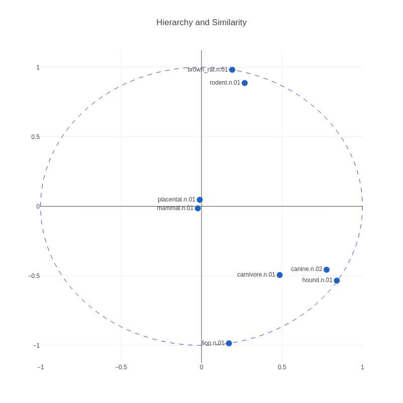
Figure 2: Positions of a sample of node vectors in 2-D space from an actual Poincaré embedding. Note that as we move toward the boundary, we begin to see nodes lower and lower in the hierarchy. Also, nodes similar to each other are close to each other.
The model achieves this by defining a loss function that penalizes low distances between unconnected nodes and high distances between connected nodes, and then training over the list of connected nodes, along with randomly sampled negative examples, using gradient descent.
The main innovation here is that these embeddings are learnt in hyperbolic space, a space that has received attention recently in network science, as it is naturally equipped to model hierarchical structures [4], as opposed to the commonly used Euclidean space. The reason presented for this is that hyperbolic spaces are more suitable for capturing hierarchical information inherently present in the graph. Embedding nodes into a Euclidean space while accurately preserving the distance between the nodes usually requires a very high number of dimensions.
An important point to note in the visualizations above is that the actual distance between two nodes is not the same as the "naked-eye distance" that can be seen. The actual distance is the Poincaré distance, whereas the "naked-eye distance" is the Euclidean distance. To get a better sense of Poincaré distance, another visualization is presented below:


Figure 3 (click to zoom): Heatmap showing the Poincaré distances from the red point to all points in a unit circle.
From this visualization, we can observe a couple of things:
- Distances increase much more quickly when the origin point is closer to the boundary – this can be seen visually from the fact that the darker region around the origin point grows smaller and smaller. This is also borne out from the mathematical formula for Poincare distance.
- For points close to the boundary, Poincare distance to other points close in Euclidean terms is relatively low, but then increases significantly and saturates – this explains the positioning of children of a parent node close to the boundary in a small arc around the parent node, and the presence of all negative nodes to the parent node outside of that small arc.
2. The journey of implementation
2.1 Datasets and other implementations
The paper makes use of the following datasets to train and/or evaluate a Poincaré model:
- WordNet noun hierarchy [2]
- HyperLex [3]
- Scientific collaboration networks (AstroPh, CondMat, GrQc, HepPh)
Thankfully, all of these datasets are publicly available, removing one of the more significant hurdles often encountered while replicating research papers.
The authors haven't published a reference implementation yet (they have mentioned to us over email that they do plan do so), but we found a couple of independent open source implementations:
Our first idea was to evaluate these implementations to see how they did on the evaluation tasks described in the paper. The NumPy implementation had to be modified slightly to be able to use it with our own hyperparameters and user-specified data. In addition, we discovered a few errors in it, which we fixed and then evaluated. We also made some changes to the C++ implementation in order to use "burn-in", a unique initialization method described in the paper.
After evaluating these implementations, we found that we couldn't achieve great results with the NumPy implementation, however the C++ implementation gave us fairly reasonable results. The results below are on the WordNet Reconstruction task from the paper, described in more detail in this detailed evaluation notebook:
| Task: WordNet Reconstruction | Dimensions | |||||
|---|---|---|---|---|---|---|
| Model Description | 5 | 10 | 20 | 50 | 100 | 200 |
| C++: burn_in=0, epochs=200, eps=1e-06, neg=20, threads=8 | 191.69 0.34 |
97.65 0.43 |
72.07 0.51 |
55.48 0.57 |
46.76 0.59 |
49.62 0.59 |
| C++: burn_in=0, epochs=50, eps=1e-06, neg=20, threads=8 | 265.72 0.28 |
116.94 0.41 |
90.81 0.49 |
59.47 0.56 |
55.14 0.58 |
54.31 0.59 |
| Numpy: epochs=50, neg=20 | 9617.57 0.14 |
5902.65 0.16 |
3868.78 0.19 |
1117.77 0.25 |
529.92 0.30 |
377.45 0.35 |
Table 1: Mean rank and MAP (Mean Average Precision) for the C++ and NumPy implementations on the WordNet Reconstruction task for different model sizes and hyperparameters.
2.2 Beginning the Gensim implementation
So, we decided to write our own implementation as part of Gensim. Our plan was to follow the C++ implementation as an initial reference point, as both the code quality and the results seemed fairly solid, and then once we'd achieved the same results, move on to improving them further to match the paper. We decided on using NumPy for the initial implementation instead of more featured machine learning libraries like Tensorflow or PyTorch, for 2 reasons:
- The model uses a variant of SGD called Riemannian Gradient Descent, and we were unsure if implementing this was easily doable in the above libraries. NumPy on the other hand gives us the flexibility to do so, although at the cost of figuring out how to compute the derivatives ourselves.
- We didn't want to create new major dependencies for Gensim without a meaningful reason to do so.
We also decided to use autograd, a nifty Python library that computes the derivatives of a function defined in terms of NumPy operations. Autograd was too slow to use for actually computing the gradients during training, however it was super-useful for performing automated verification of the gradient calculations written by us ourselves, giving us confidence in the correctness of our calculations, and therefore letting us iterate quickly.
A pure NumPy implementation can be slow, because NumPy does a significant amount of dynamic memory allocation internally for temporary arrays, which has a direct time-cost, as well as the indirect cost of ruining caches. Our plan was to get a correct implementation first, and then optimize the hotspots with Cython and BLAS (similar to the word2vec optimization in Gensim).
Once we began our implementation, we discovered a fair amount of differences in the C++ implementation from the paper.
2.3 Loss functions and partial derivatives
The paper mentions this loss function:

where  is the set of negative examples for
  .
.
The denominator consists of terms involving the distance between node and negative examples of nodes  for .
for .
However, the C++ implementation makes use of a slightly modified loss function:

where the denominator also includes the term from the numerator:  .
.
This more closely resembles a traditional softmax log-loss function. The gradients used to update the vectors depend on this choice of loss function. We attempted both variants of the loss function and the corresponding partial derivatives, and found that the softmax-like loss function yielded better results.
Note that negative sampling is used while training, as mentioned in the paper, since training over all the negative examples from the dataset is not computationally feasible.
2.4 Non-uniform negative sampling
We were a fair way off from the C++ results, and we weren't sure why this was the case. It turned out that, under the hood of the rather misleadingly named UniformNegativeSampler, the underlying random number generator std::discrete_distribution was being initialized with the counts of how many times each node occurred in the dataset. Therefore, more common nodes were more likely to be chosen as negative examples, and therefore far more updates were likely to be performed on these nodes, affecting the final vectors significantly.
The paper mentions uniform negative sampling too, which is why this wasn't detected earlier. Using weighted negative sampling helped us achieve the same results as the C++ implementation.
2.5 Into (sort of) unexplored territory
We'd finally achieved the same results as the C++ implementation, however we were still quite some way off from the results in the paper. The following were the changes we made that helped us exceed the C++ quality and get closer to the final results.
2.6 Excluding positive edges from negative sampling
The C++ version implements negative sampling simply as weighted sampling from the entire list of nodes in the dataset. Crucially, this can potentially select positively connected nodes to the input node as a negative example, causing the connected nodes to move away from each other, which is undesirable. The simple solution is to discard the positively connected nodes from the nodes to be sampled from before sampling. However, in combination with non-uniform weights, this is difficult to implement in a performant way.
The method we used was:
- Sample (with repetitions) a large buffer of candidate nodes based on their frequency distribution
- Fetch the required number of negative examples from this buffer; if the buffer is empty, perform (1) again
- If the fetched nodes have any duplicates, or any positively connected nodes to the target node, discard them and perform (2) again.
The reason this works well is that the probability of a duplicate or positively connected node being present in the fetched sample is usually fairly low, and also because generating a large buffer of samples a few times is much faster than generating smaller samples a large number of times. In the process, we also discovered a useful trick with random sampling in NumPy:
Random #Numpy tip:
— Radim Řehůřek (@RadimRehurek) November 9, 2017
Avoid "np.random.choice" for sampling elements with probabilities, where performance matters. Too much overhead. Here 17x SLOWER than simple cumsum+searchsorted: pic.twitter.com/hKFObqPHCq
2.7 Batchwise training
Over email, the paper authors mentioned that they were using mini-batches of sizes 10-50 for gradient descent, and that smaller batches lead to better results. The paper does not mention batch-wise training, and the C++ version trains one example at a time. We implemented batch-wise training – this did not significantly change the evaluation results, however the faster computations did allow us to train on more epochs and iterate faster.
2.8 Burn-in
The paper describes a rather unique method (to the best of our knowledge) of initializing the vectors before training, which the authors call "burn-in". Basically, this involves initializing the vectors to a uniform distribution and then training with a much reduced learning rate for a few epochs. The rationale is that this results in a better initial angular layout of the vectors and reduces the sensitivity of the final vectors to a possibly "unlucky" random initialization. This did not seem to work well in practice for us at first, however after implementing the next step (L2 regularization), burn-in significantly improved results.
2.9 L2 regularization
For debugging, we'd been training 2-D Poincaré embeddings on a subset of the WordNet noun hierarchy, and visualizing the embeddings in 2-D Euclidean space (thanks to the authors for this suggestion). These were the results we'd been obtaining:
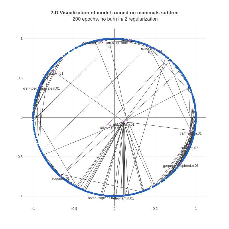
We noticed that almost all of the vectors were too close to the boundary (the vectors are constrained to a unit norm via clipping). This makes sense mathematically, as Poincaré distances near the boundary change extremely fast, and therefore it is easier for the optimizer to achieve a lower loss. However, this is essentially a form of overfitting – our goal is to obtain useful representations, not simply achieve the minimum loss value.
It seemed to us that the nodes higher in the hierarchy (often parent nodes in the set of edges) should be closer to the origin, and the nodes lower in the hierarchy (often child nodes and leaf nodes) should be closer to the boundary. A mathematical way to enforce this was by adding penalties on the norm of the parent node in an edge via L2 regularization. Note that L2 regularization is often used for all parameters, however we're only using it for the parent node in a training example. After adding L2 regularization, the results looked a lot more reasonable:
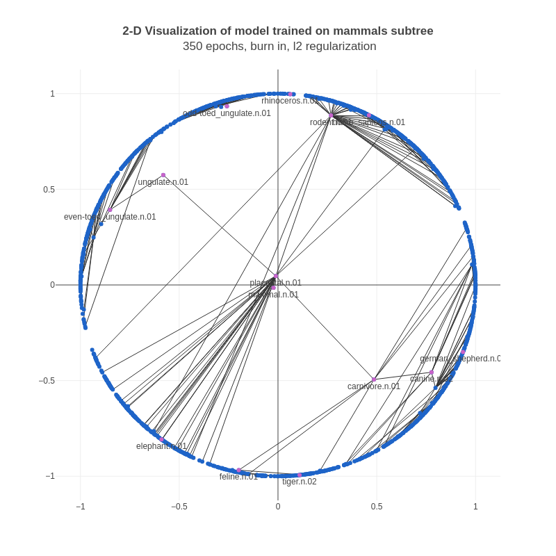
Here, the nodes with a large number of children are further away from the boundary than above. Also, the positive edges for these nodes are focused in much smaller arcs, and aren't scattered around the whole circle like in the previous example.
3. Final results
The following are the results we obtained for the WordNet Reconstruction task, where we evaluate two correlated metrics – Mean Average Precision and Mean Rank.
Our results:
| Task: WordNet Reconstruction | Dimensions | |||||
|---|---|---|---|---|---|---|
| Model Description | 5 | 10 | 20 | 50 | 100 | 200 |
| C++: burn_in=0, epochs=200, eps=1e-06, neg=20, threads=8 | 191.69 0.34 |
97.65 0.43 |
72.07 0.51 |
55.48 0.57 |
46.76 0.59 |
49.62 0.59 |
| C++: burn_in=0, epochs=50, eps=1e-06, neg=20, threads=8 | 265.72 0.28 |
116.94 0.41 |
90.81 0.49 |
59.47 0.56 |
55.14 0.58 |
54.31 0.59 |
| Gensim: batch_size=10, burn_in=0, epochs=50, neg=20, reg=0.0 | 154.41 0.40 |
62.77 0.63 |
27.32 0.72 |
20.22 0.77 |
16.15 0.78 |
13.20 0.79 |
| Gensim: batch_size=10, burn_in=10, epochs=200, neg=10, reg=1 | 61.48 0.38 |
54.70 0.41 |
53.02 0.41 |
50.80 0.42 |
49.58 0.42 |
48.56 0.43 |
| Numpy: epochs=50, neg=20 | 9617.57 0.14 |
5902.65 0.16 |
3868.78 0.19 |
1117.77 0.25 |
529.92 0.30 |
377.45 0.35 |
Table 2: Mean rank and MAP (Mean Average Precision) for the Gensim, C++ and NumPy implementations on the WordNet Reconstruction task for different model sizes and hyperparameters.
Results as reported in the paper:
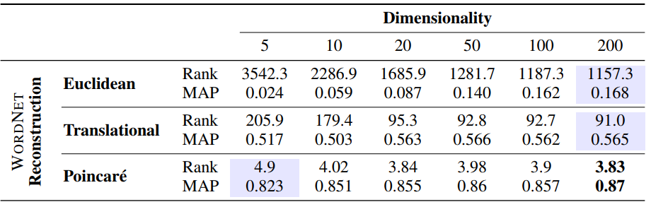
We see that we still have some way to go to match the original results reported in the paper, especially for lower dimensional embeddings. However, we’re much closer for higher dimensional embeddings, while also significantly outperforming previous state-of-the-art results as well as the results of Poincaré embeddings from other open source implementations.
On the Lexical Entailment task from HyperLex [3], these are the results -
| Lexical Entailment (HyperLex) | Dimensions | |||||
|---|---|---|---|---|---|---|
| Model Description | 5 | 10 | 20 | 50 | 100 | 200 |
| C++: burn_in=0, epochs=200, eps=1e-06, neg=20, threads=8 | 0.45 | 0.46 | 0.45 | 0.45 | 0.45 | 0.46 |
| C++: burn_in=0, epochs=50, eps=1e-06, neg=20, threads=8 | 0.44 | 0.43 | 0.47 | 0.44 | 0.45 | 0.44 |
| Gensim: batch_size=10, burn_in=0, epochs=50, neg=20, reg=0.0 | 0.47 | 0.45 | 0.47 | 0.47 | 0.48 | 0.47 |
| Gensim: batch_size=10, burn_in=10, epochs=200, neg=10, reg=1 | 0.52 | 0.51 | 0.51 | 0.51 | 0.52 | 0.51 |
| Numpy: epochs=50, neg=20 | 0.15 | 0.19 | 0.20 | 0.20 | 0.24 | 0.26 |
Table 3: Spearman's rank correlation for the Gensim, C++ and NumPy implementations on the HyperLex Lexical Entailment task for different model sizes and hyperparameters.
These are the results from paper (for Poincaré Embeddings, as well as other embeddings from previous papers) -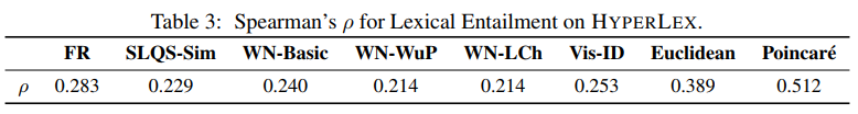
On this task, we achieve very similar results as the paper with the Gensim implementation. However, there are a few ambiguities and caveats -
- The paper does not mention which hyperparameters and model size have been used for the above mentioned result. Hence it is possible that the results are achieved with a significantly lower model size than the one we use, which would imply that our implementation still has some way to go.
- The same word can have multiple nodes in the WordNet dataset for different senses of the word, and it is unclear from the paper how to decide which node to pick. For the above results, we have gone with the sane default of picking the particular sense that has the maximum similarity score with the target word.
- Certain words in the HyperLex dataset seem to be absent from the WordNet data - the paper does not mention any such thing. Pairs containing missing words have been omitted from the evaluation (182/2163).
4. Conclusion and Next Steps
In conclusion, dealing with all these challenges was extremely enjoyable, and the journey resulted in a model that finally looks practically useful. We still have some way to go:
- Optimizing the training using Cython/BLAS for the hotspots.
- Matching the exact results from the paper (elusive despite direct email communication with the authors and trying everything we could think of).
- Decreasing memory requirements; right now the model requires memory linearly proportional to the number of edges in the dataset. Gensim is built on the idea of document streaming, as requiring the entire dataset to be in RAM limits scalability. This leaves room for implementing Poincaré embeddings using online training.
5. References
[1] Maximilian Nickel and Douwe Kiela. Poincaré embeddings for learning hierarchical representations, 2017.
[2] George Miller and Christiane Fellbaum. Wordnet: An electronic lexical database, 1998.
[3] Ivan Vulic, Daniela Gerz, Douwe Kiela, Felix Hill, and Anna Korhonen. Hyperlex: A large-scale evaluation of graded lexical entailment, 2016.
[4] Dmitri Krioukov, Fragkiskos Papadopoulos, Maksim Kitsak, Amin Vahdat, and Marián Boguná. Hyperbolic geometry of complex networks, 2010.
