 RARE Technologies
In my previous post on the new open source Python Bounter library we discussed how we can use its HashTable to quickly count approximate item frequencies in very large item sequences. Now we turn our attention to the second algorithm in Bounter, CountMinSketch (CMS), which is also optimized in C for top performance.
(Shoutout to dav009 who already ported our CountMinSketch to Golang and provided some extra measurements.)
A Data Structures Refresher: CountMinSketch
Count-min sketch is a simple yet powerful probabilistic data structure for estimating frequencies (also called counts) in very large datasets of elements (aka objects), closely related to Bloom filters. Wikipedia provides an excellent overview of the CMS algorithm. There are also several other resources out there that can help you get the idea, including this site dedicated to the algorithm and several great blogs.
In short, you can visualize CMS as working over a two dimensional “table” of cells called “buckets”. This table has depth rows and width columns. Each bucket in the table stores a single number. Any element to be processed by CMS is mapped to depth different buckets, one bucket per row. Which bucket gets mapped in each row is calculated using hashing: we hash the input object using a row-specific salt, to make the hash functions row-wise independent. Then to increment that object’s count, we increment the value of each of its mapped buckets. To get the object’s (approximate) count later, we find the minimum value across all its mapped buckets. That’s it!
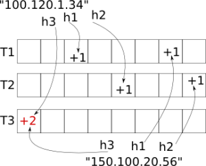
Inserting two objects, the strings "100.120.1.34" and "150.100.20.56" into a Count-Min Sketch table of depth=3 and width=8. Note the collision in the bottom-left bucket. Image courtesy of L. Kozma.
What about hash collisions? Clearly, two different objects can end up mapping to one or more of the same buckets. The nice approximative properties of CMS stem from the fact that we expect objects that collide in one row not to collide in a different row.
Given an object, the value in each bucket is an overestimation of its frequency count: it can be larger than the real count (due to a collision), or equal to it (no collision), but it can never be smaller. We can also say that there is a bias in one direction (up).
The CMS count for an object is estimated by retrieving the mapped bucket values from each row and returning the smallest of these numbers. This will be the one closest to the real value (though still possibly overestimated). With more rows, we have a better chance of finding a bucket that has had no collision, or at least find one where the error from overestimation is the smallest.
To improve on this basic idea, Bounter always uses the conservative update heuristic. While incrementing, after finding the appropriate bucket in each row, only those buckets that share the lowest value are updated (the remaining buckets must already have been affected by a collision and overestimated). This significantly mitigates the collision error and greatly improves the overall precision of the algorithm, compared to the basic version.
On top of this algorithm, for user convenience, Bounter adds a HyperLogLog structure to estimate the overall number of distinct elements inserted into the CMS table so far, and also maintains a precise tally of all these elements.
Usage
To initialize CountMinSketch, use either one of these methods:
from bounter import bounter, CountMinSketch

# if you don't need key iteration, Bounter chooses the CMS algo automatically
counts = bounter(need_iteration=False, size_mb=256)

# or you can choose it explicitly yourself
counts = CountMinSketch(size_mb=256)  # specify max memory, table size calculated automatically
counts = CountMinSketch(width=8388608, depth=8)  # specify concrete table size

counts.size()  # print overall structure size in bytes
268435456
counts.width  # buckets per table row
8388608
counts.depth  # number of table rows
8
Count frequencies just like with HashTable:
counts.update(['a', 'b', 'c', 'a'])
counts.increment('b')
counts.increment('c', 2)   # larger increments work too!
print(counts['a'])
2
CountMinSketch does not support iteration of elements. This is because the keys (the objects themselves, or their hashes) are never stored. The += syntax for increment is also unsupported. This is because assignment is unsupported, and Python treats += only as shorthand for calling __getitem__, incrementing the result, and feeding it into __setitem__.
The depth parameter
By increasing the depth parameter, you can increase the chance of avoiding a collision in at least one row and thus improve the accuracy of the results. However, this also increases the table size and the processing time of each insert or count operation. In our experiments, we had the best results with depths between 8 to 16, meaning we used 8-16 different hashes per object. Above that, investing memory into additional width (as opposed to depth) yields a much better marginal improvement.
Logarithmic counters
Each bucket of the standard algorithm takes 32 bits, and is thus able to represent object counts between 0 and 4,294,967,295. Bounter also implements approximate counting in the buckets, reducing the size of each bucket while extending the value range. The idea of approximate counting is to represent a range of values with a single counter value, stepping to the next value only sometimes, probabilistically. For instance, to step from the bucket value 5 (representing object counts of 32-63) to 6 (representing 64-127), we need to pass a random test with a 1/32 chance of success. This means we need an average of 32 attempts to take this one step.
This "base-2" setup of doubling the range and halving the probability makes for an intuitive example, but base-2 would be too crude and imprecise for Bounter. In reality, we use the same principle but with a lower base: we take more steps between each power of 2 (8 or 1024 steps). So, as an example with 8 steps, we would step from count range 32-35 (represented by bucket value 24) to 36-39 (25) with p=1/4, then to 40-43 (26) with p=1/4, and so on with the same p until 64-71 (32), from which we would step to 72-79 (33) with p=1/8.
counts = bounter(need_iteration=False, size_mb=254, log_counting=1024)
counts = bounter(need_iteration=False, size_mb=254, log_counting=8)
Log1024 is a 16-bit counter which is precise for values up to 2048. Larger values are off by ~2%. The maximum representable value is around 2^71.
Log8 fits into just 8 bits and is precise for values up to 16. Larger values are off by ~30%, with the maximum representable value around 2^33.
Using these counters introduces a different kind of error. We call it the "counter error", as opposed to "collision error" which comes from bucket collisions. Unlike the collision error, the counter error is unbiased. Also, while collision errors affect primarily small values, the counter error only occurs for larger values. By using approximate counters, we can trade some of the collision error (freeing up to 4x more buckets in the same space) for the counter error.
So much for theory. Let us look at some measurements and their visualisations to better understand the trade-offs we are making.
Evaluation
We use the same setup as the last time with HashTable: First, we count all word bigrams across all ~4 million articles from the English Wikipedia. Then, we use their counts to determine phrase collocations and calculate the resulting precision, recall and F1 values for this task.
We include the Hashtable results from the last part in the visualisations, so that you can directly compare against its results.
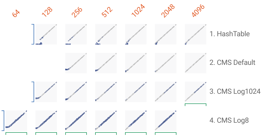
You can see these accuracy charts in action and inspect individual errors (shades of blue) interactively, using Google's awesome FacetsDive tool. Click here to open the plot above in a new, interactive browser window.
With limited memory, each algorithm produces a characteristic error, which is best understood when looking at the Facets visualisation and inspecting the concrete examples there.
Just as with HashTable, you can use the quality() function to get the ratio of the cardinality of the inserted items to the CMS capacity (total number of buckets). For a quality near or below 1, the results show no collision error.
The following table hints at the relationship of Quality (the number returned by quality(), the first number in the table) and F1 score (the second bold number in the table, higher is better, 1.0 is perfect) for several combinations of counter algorithms and RAM footprint. The blank cells represent combinations which were not tested.
As you can see, we can reach (or get very close) to the perfect F1 score of 1.0 with Quality values around 3.
| Used RAM Algorithm |
64 MB | 128 MB | 256 MB | 512 MB | 1024 MB | 2048 MB | 4096 MB |
|---|---|---|---|---|---|---|---|
| HashTable | 42.78 0.917 | 21.39 0.952 | 10.69 0.978 | 5.34 0.996 | 2.67 1.0 | 1.34 1.0 | |
| CMS Default | 21.76 0.821 | 10.88 0.993 | 5.44 0.998 | 2.72 1.0 | 1.36 1.0 | ||
| CMS Log1024 | 21.76 0.818 | 10.88 0.987 | 5.44 0.993 | 2.72 1.0 | 1.36 0.995 | 0.68 0.998 | |
| CMS Log8 | 21.76 0.784 | 10.88 0.960 | 5.44 0.967 | 2.72 0.969 | 1.36 0.975 | 0.68 0.974 |
CMS Quality score and F1 score on the task of collocation detection in the English Wikipedia, using CMS to represent the raw n-gram counts. Python's built-in Counter would occupy 17.2 GB to count all 179,413,989 distinct word pairs exactly (100% F1 score).
For the specific task of determining collocation phrases, HashTable is a clear winner. This is because the specific type of numerical error it produces (discarding the long tail) is a good match for the task, since low-counts objects are irrelevant. As Quality climbs over 2, Hashtable already pins the majority of the long tail to 0.
On the other hand, CountMinSketch manages to estimate even the elements of the long tail with great precision while Quality remains in the single digits. You can see this property quite well in the visualisation. This makes the CMS variants more appropriate when you are interested in the long tail of element counts.
Conclusion
Our advice to "power-users" of Bounter is the following: use the HashTable or CMS algorithms with default settings, using the amount of memory you have available, then consult the quality() number. If this number is very high (over 5), using the log1024 or log8 variant of CMS might improve your results. If the number is less than 1.0, there should not be any error in the results at all and you can safely lower the amount of RAM in the size_mb parameter (if you care about memory). For example, with a Quality rating of ~0.1, you can assign 8x less RAM to Bounter.
If you have enough memory for now, how do you choose between CountMinSketch and HashTable? Think about the kind of estimation error that matters to your application. Is it critical to never report positive occurrences for an object you never saw (avoid CountMinSketch)? Or to never report 0 for objects you saw only rarely (avoid HashTable)? This is the primary trade-off between false positives and false negatives.
HashTable has a discrete threshold given by its capacity. Until it is filled, it is guaranteed to be 100% accurate. When the capacity is used up, or even exceeded by more than 2x, it is guaranteed to misrepresent all the elements that did not fit in, cutting the long tail. On the other hand, CountMinSketch has a tiny probability of an overestimation error to begin with, and this continuously increases as you fill it with more values. In practice, CountMinSketch rate of error remains small enough even when its size is exceeded by 2-10x. Thus, it trades simplicity of its guarantees for a much better overall accuracy of the entire distribution.
Hopefully, our articles helped you understand the algorithms for approximate counting and navigate their trade-offs, letting you make the right decisions for your application.
Good luck with your counting and let us know in the comments if you found some nice use for our library!
See also
-
Our tutorial series on interactive analytics in browser & confusion matrix inspection with Facets Dive.
-
Tutorial on data streaming with Python.
